Virtualization Performance Testing

Virtualization technologies (such as VMware, Parallels, Xen, KVM, Waratek, etc.) have become very popular for good reasons, including but not limited to the following:

• Application density can be increased
• Server resource usage can be maximized
• Hardware costs can be reduced many-fold
• The number of servers required to run the same load can be reduced
• Applications become more portable

It is critical to do performance, load, and stress testing of a virtualization solution before rolling it out for several reasons:

• Different applications behave differently in a virtualized environment and some are more suitable than others
• Performance or stability could be affected in a virtualized environment
• Virtual machine sizing can drastically affect application behavior
• Application configuration can be different when run in a virtualized environment.

This post gives a brief outline of how to do performance, load and stress testing of a virtualization solution.

1. Include online and batch test cases as well as administrative operations
2. Test bare metal (physical server) as a baseline to be compared to virtualization results
1. See how many instance of the application can be run on bare metal
2. Push bare metal up to server capacity
3. Test virtualization
1. Run VMs on the same bare metal server or an equivalent one
2. Push one VM up to capacity, then two VMs, then three VMs, etc., up to the highest density desired.
3. Capture hypervisor server resource usage metrics (cpu, memory, disk, network)
4. Verify that VM performance compares reasonably relative to bare metal
5. Verify that VM capacity compares reasonably relative to bare metal
6. Verify that VM application stability compares reasonably relative to bare metal
7. If performance or stability is not acceptable, see if application tuning is needed or virtual machine tuning is needed.
8. Include stability tests in which high load is applied for an extended period of time.
9. Perform administrative operations while system is under high load.
10. Once performance and stability are acceptable, publish the results and the tuning and configuration needed to achieve acceptable results.

Performance Testing ROI and Black Swans

What return on investment/ROI can be expected from performance testing?  There are two categories of "return" for performance and stability testing.

One category of return is a simple, quantifiable return in which performance testing results allow the amount of hardware required to be reduced in a couple of ways:

• Application tuning and optimization allowing the same amount of hardware to handle additional traffic
• Proof of hardware overcapacity, showing that a reduced amount of hardware would be sufficient to handle peak traffic, allowing hardware inventory to be reduced  

The second category of return is not a return so much as an insurance policy, or protection against a fat tail or black swan event.  In this case, you are protecting yourself against system stability bugs whose consequences can be absolutely catastrophic, up to the complete destruction of the business.

Consider the example of Knight Capital's botched software rollout on August 1st, 2012.  The rollout triggered unexpected trades that cost the firm $440 million, depleting its operating capital.  This weakened position allowed outside investors to take a controlling 70% stake in the company as terms of its bailout.

By doing performance and stability testing, catastrophic stability bugs may be missed due to limitations of the test environment or test data, or failure to anticipate the nature of production behavior leading to the disaster.  However, if a catastophic stability bug is discovered and fixed, which happens regularly, a black swan event has been quietly and successfully sidestepped.  The value is avoiding a devastating black swan event that brings down the company through loss of customers, loss of reputation, lawsuits, takeovers, etc.  Not to mention more individual losses such as loss of job, bonus, promotion, career, etc.  The cost of the testing is fixed and predicable, simply the cost of supporting ongoing performance testing, in effect the insurance policy premiums protecting against the black swan.

How to Performance Test in a Service-Oriented Architecture

How do you performance test, stress test, and load test in the world of service-oriented architecture (SOA)?

The answer is that you test it at different levels of granularity, typically three levels.  One, obvious level is the service.  Another level is end to end.  The third level is the module level, the low-level building blocks making up the service.

One necessary precondition to adequate performance testing services is proper instrumentation providing key performance metrics.  Response times, transaction rates, and and success/failure counts must be available for all service entry points and downstream calls.  This allows response time contributions to be allocated accurately to the proper services and allows fast performance problem debugging.

The three layers of SOA performance testing share the following in common.

• Scalability Testing
• What is capacity?
• What bottleneck is limiting capacity?
• What is response time at various loads?
• What is the canonical performance chart?

• Stability Testing
• Is the application stable?
• Is the application fault tolerant?

• Performance Regression Testing
• Does performance degrade from build to build?
• Does server resource usage increase from build to build?

• Metrics on server resource usage
• CPU
• Memory
• Network
• Disk

Module level SOA performance testing is done as follows:

• Test key functional code paths at module level
• Use multi-threaded, concurrent execution
• Run within unit test framework
• Run within continuous integration framework
• Run frequently, each check-in, build, or version

Service level SOA performance test is done as follows:

• Test through public entry point
• Isolate service under test from other services
• Use spoofing or stubbing of backend services, mimicking their response time behavior
• Determine response time and availability service level agreements (SLAs) based on test results
• Thoroughly test the clustering or load balancing mechanism used to scale the service out horizontally.

End to end level SOA performance test is done as follows:

• Test public entry point into the application
• Verify that bottlenecks hit are consistent with capacity of individual services discovered in service-level testing.
• Verify fault tolerance of unavailable downstream services

An additional layer is infrastructure testing.  This could include messaging infrastructure, caching infrastructure, storage infrastructure, database infrastructure, etc.  Key infrastructure should be directly tested for scalability and stability in some cases to ensure that it behaves as expected and scales as expected.

SOA performance testing can be summarized in the following conceptual chart:

Using Loadrunner Pacing to Hit a Specific Transaction Rate

It is often necessary to apply load at a specific transaction rate per second (TPS).  For example, it may be necessary to test every build or patch of an application by running a fixed benchmark of 20 queries per second against the application, measuring the response time and server utilization at that fixed load.  By then examining the trend over time of response time and server resource utilization under uniform load, performance regressions can be easily identified.

One way to set a specific transaction rate using Loadrunner is by using the pacing feature.

Pacing specified how often an iteration starts.  For example, if an iteration runs in 300 - 500 milliseconds, setting pacing to 1 second for that script will case a user to run the iteration once every second as illustrated below:

Each second the iteration starts and then ends after 400 ms or so.  At the next second interval, the next iteration starts.  An exact transaction rate of 1 iteration per second is reached in this way.  By increasing the user count in this case to 10, a transaction rate of 10 TPS can be achieved.  

An iteration can have multiple transactions per iteration.  If the above example was an iteration that included three transactions (query1, query2, and query3), a single user would run three transactions per second and 10 users would give 30 TPS.

The following formula provides a calculator for determining what the pacing in seconds should be set to given three input parameters, transactions per iteration, user count, and target transaction rate:

• transactionsPerIteration  (the number of transactions included in an iteration)
• users (the number of users to be run)
• tps (the target transaction rate per second)

For example, suppose transactionsPerIteration = 3, users = 50, and target transaction rate = 10 TPS.  The equation gives a pacing in seconds of (3 * 50)/10 = 1.5 seconds.

One thing that can prevent the target transaction rate from being reached is when the iteration slows down when run under multiple users such that the time an iteration runs is longer than the pacing time.  In this case a warning is generated and the transaction rate is not reached.  This can be sometimes be avoided by increasing the user count somewhat.

However, the problem could also be due to limitations in the application's vertical scalability.  The application may have concurrency problems preventing concurrent users from executing the transaction without blocking other users.  In a worst case, the application's concurrency problems may make it impossible to reach the target transaction rate regardless of the number of users.  In any case, it is worthwhile to investigate what the bottlenecks are that are limiting scalability and resolving those issues.

networkspeedtest - a free network bandwidth test application

Download

Network performance problems can cause a variety of difficult to diagnose application performance problems.  It can be necessary to test the bandwidth of the network to verify whether the bandwidth is as expected.
Network speed test is a free, simple network test application that will copy files from one test server to another, showing the network bandwidth used in bytes per second.  This could be compared to a previous baseline to show a network problem.  For example, if 50 MB/sec of bandwidth was previously seen between two test servers, and now there is 1 MB/sec between the same two test servers, there is likely a network problem.

Installation
Unzip networkspeedtest directory to c:\temp


USAGE
copyto <SERVERNAME> repeat

(Copies current directory to SERVERNAME\c$\temp\networkspeedtest showing network speed in bytes per second.)
(repeat parameter causes it to repeat the operation indefinitely)


EXAMPLE
(Shows network bandwidth of 48 MB/sec from current server to SERVER1)

C:\Temp\networkspeedtest> copyto SERVER1 repeat

-- Speed of copying files of varying sizes to SERVER1 in bytes per second
    Speed :            48339531 bps.
    Speed :            58255333 bps.
    Speed :            41308327 bps.
    Speed :            48339531 bps.
    Speed :            48339531 bps.
    Speed :            48339531 bps.
    Speed :            48339531 bps.
    Speed :            48339531 bps.
    Speed :            48339531 bps.
    Speed :            48339531 bps.
    Speed :            41308327 bps.
    Speed :            58255333 bps.
    Speed :            48339531 bps.
    Speed :            41308327 bps.

The following shows windows task manager networking tab during this test:

VisualCSV - A Free CSV Analyzer - CSV File to Chart, CSV File to Stats, CSV File to Histograms, CSV File Correlation Charts

VisualCSV         Download Now

VisualCSV is a free CSV analyzer that is:

• A Java application 
• Converts CSV File to Charts
• Converts CSV File to Statistics
• Converts CSV File to Histograms
• Converts CSV File to Correlation Charts

Performance testing, system monitoring, etc. often generate CSV files that must be analyzed, and typically you need to chart columns, calculate stats on columns, correlate columns, etc.

VisualCSV is a java application that, given a csv file input, will generate most of the data you need automatically, including:

• statistics on each column in the CSV file 
• min
• avg
• max
• standard deviation
• variance, median
• percentiles (such as 95th and 98th percentiles, or any list of percentiles you specify)

• trend charts for each column in jpeg format
• histogram charts for each column
• correlation metrics between any pairs of columns
• correlation charts showing correlations between any pairs of columns
• transposed correlation charts reversing x and y axis.
• charts created using jfreechart
• stats created using apache commons math

The following sections shos sample output generated from processing a csv file from windows performance monitor (perfmon) having the following columns:

(PDH-CSV 4.0) (Pacific Standard Time)(480)

\\CHELSTRPL006\Memory\Available Bytes

\\CHELSTRPL006\Network Interface(HP NC382i DP Multifunction Gigabit Server Adapter _4)\Bytes Total/sec

\\CHELSTRPL006\Network Interface(HP NC382i DP Multifunction Gigabit Server Adapter _4)\Output Queue Length

\\CHELSTRPL006\PhysicalDisk(_Total)\% Disk Time

\\CHELSTRPL006\PhysicalDisk(_Total)\Avg. Disk sec/Read

\\CHELSTRPL006\PhysicalDisk(_Total)\Avg. Disk sec/Write

\\CHELSTRPL006\Processor(_Total)\% Privileged Time

\\CHELSTRPL006\Processor(_Total)\% Processor Time

Summary stats

The following csv file showing summary stats for each column is generated.

Trend Charts

For each column, a chart is generated such as this:

Histograms

For each column, a frequency histogram showing number of occurrences by bucket is generated such as this:

The number of buckets is configurable.

For each chart, a relative frequency histogram  is generated showing relative frequency by bucket is generated such as this:

Correlations Between Columns

For each pair of columns, a csv file showing correlations between pairs of columns is generated such as this:

Correlation Charts

For each pair of columns, a correlation chart and a transposed correlation chart (x and y swapped) is generated such as this:

Download

VisualCSV can be downloaded here:

• https://docs.google.com/open?id=0B4gruS14dMq4N2M4ZDZjNWYtMTIzYy00NmRmLWJiNTYtOWVhYTc4NjJiMWU2

Usage

• VisualCSV requires java in the system path.  It has been tested with java 1.6 and probably runs fine with 1.5 and 1.7 as well.
• Download and unzip the files.
• Analyze the sample CSV file from command line by running:
• run.bat TestPerfmonFile.csv
• This will analyze the test file and generate output in directory .\out.  The output should 

Configuration

Client configuration is found in the file client.config.

Columns can be specifically included or excluded by putting them in specified include or exclude files which by default (as specified in client.config) are called 

Column-Include-Names.properties

Column-Exclude-Names.properties

The include file can be empty or missing in which case all columns are analyzed.  Otherwise, the columns analyzed are all columns in the include file minus those in the exclude file.

Likewise columns can be specifically included or excluded from being correlated with each other by putting them in specified include or exclude files which by default (as specified in client.config)  are called 

Correlation-Include-Names.properties

Correlation-Exclude-Names.properties

Again, the include file can be empty or missing in which case all columns are correlated. Otherwise, the columns in the exclude file are subtracted from the includes.

The client.config file includes the following values by default:

# --- Functionality
createTrendCharts=true
computeCorrelations=true
createCorrelationCharts=true


# --- whether to include or exclude columns from analysis
# --- put columns in this file to include them in analysis.  empty file or no file means analyze all columns.
columnIncludeFile=Column-Include-Names.properties


# --- put columns in this file to exclude them from analysis.
columnExcludeFile=Column-Exclude-Names.properties


# --- whether to include or exclude columns from correlation with other columns
correlationIncludeFile=Correlation-Include-Names.properties
correlationExcludeFile=Correlation-Exclude-Names.properties




# --- Timestamp column index (0 = first column)
hasTimestampColumn=true
timestampColumnIndex=0


# --- Java SimpleDateFormat date format for parsing timestamps
timestampFormat=MM/dd/yyyy HH:mm:ss.S

# Letter Date or Time Component Presentation Examples
# G Era designator Text AD
# y Year Year 1996; 99
# M Month in year Month July; Jul; 07
# w Week in year Number 27
# W Week in month Number 2
# D Day in year Number 189
# d Day in month Number 10
# F Day of week in month Number 2
# E Day in week Text Tuesday; Tue
# a Am/pm marker Text PM
# H Hour in day (0-23) Number 0
# k Hour in day (1-24) Number 24
# K Hour in am/pm (0-11) Number 0
# h Hour in am/pm (1-12) Number 12
# m Minute in hour Number 30
# s Second in minute Number 55
# S Millisecond Number 978
# z Time zone General time zone Pacific Standard Time; PST; GMT-08:00
# Z Time zone RFC 822 time zone -0800


# --- chart settings
chartEveryNthDataPoint=1
histogramLogScale=false


# --- statistics settings
createChartCorrelationGreaterThan=0.0
createChartCorrelationLessThan=-0.0
numHistogramBuckets=10
percentiles=80,90,95,98,99


# --- Output file locations
outDir=out
deleteStatsDirs=true
outTrendDir=out/Trend
outCorrelationDir=out/Correlation
outHistogramDir=out/Histogram
outputStatsFile=SummaryStats.csv

How to Test ODBC Data Sources Using Loadrunner

It can be convenient to test databases using Loadrunner to take advantage of its parameterization and other functionality.  One easy way to get started with this is to to use ODBC vuser type and record the transaction through some ODBC client.  This post describes one way to do this.

Install WinSQL Lite, which can be used for free. http://synametrics.com/SynametricsWebApp/WinSQL.jsp

Start WinSQL and configure an ODBC data source to your database.

Test the connection.
Create a new vugen script of type ODBC and choose the WinSQL as the application to launch:

Vugen will then launch the WinSQL app and connect to the database, bringing up a query window.
Enter your query in the query window and execute it:

Disconnect within WinSQL.
Stop recording within vugen.

You now have your script which can be modified, rearranged and parameterized as needed.

Monitoring Linux Servers during Performance Tests

The server resource usage of the servers used in a load or performance test should be monitored and saved to be able to later verify system bottlenecks and behavior.  Linux servers can be monitored in a number of different ways.

If you are using Performance Center to drive load, linux monitors can be enabled as part of the load test, allowing the linux metrics to be conveniently combined with other metrics in a single report.  That requires the rstat daemon to be running on the linux servers monitored.  For CentOS, rstat daemon can be installed as follows:

sudo yum install rpcbind
sudo wget http://www.wyzaerd.com/public/rpc.rstatd-4.0.1.tar.gz
sudo tar xvzf rpc.rstatd-4.0.1.tar.gz
cd rpc.rstatd-4.0.1
sudo ./configure
sudo make
sudo make install
sudo /usr/local/sbin/rpc.rstatd

Monitors can then be configured in performance center to collect stats from the linux server running rstatd.

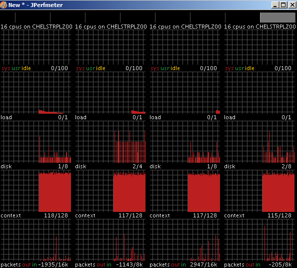
Another tool for viewing and collecting server resource usage on linux is jperfmeter (http://jperfmeter.sourceforge.net/).  Jperfmeter provides a gui view of resource usage metrics of a list of servers, showing values over time.  For example the following shows the jmeter console for a group of 4 linux servers:

The jmeter metrics can be saved to a delimited text file for later analysis:

A third tool for monitoring linux server resource usage is sar. The following script will collect server resource usage on CPU, memory, network, and disk utilization:


# Run sar every 10 seconds until stopped
# cpu
sar -u 10  > sar.cpu.log &
# free memory
sar -r 10  > sar.freememory.log &
# disk total
sar -b 10  > sar.disk.log &
# network by device
#    - Note that you need to filter by the adaptor in use.  
#    - Run "sar -n DEV 10" to see which adaptor is being used
sar -n DEV 10 |grep eth1 > sar.network.log &

On some versions of sar, it is necessary to provide a number of data points to collect such as the following:

# Run sar every 10 seconds until stopped
# cpu
sar -u 10 99999 > sar.cpu.log &
# free memory
sar -r 10 99999 > sar.freememory.log &
# disk total
sar -b 10 99999 > sar.disk.log &
# network by device
#    - Note that you need to filter by the adaptor in use.  
#    - Run "sar -n DEV 10" to see which adaptor is being used
sar -n DEV 10 99999 |grep eth1 > sar.network.log &


For a test of one or two hours, a 10 second collection interval is convenient, providing a couple of hundred data points.  For an overnight test, a 300 second collection interval is usually appropriate.

Output

The cpu log file shows user and system CPU % utilization:

03:07:55 PM     CPU     %user     %nice   %system   %iowait    %steal     %idle

03:08:55 PM     all     73.99      0.00      2.43      0.21      0.00     23.37

03:09:55 PM     all     81.79      0.00      2.67      0.21      0.00     15.34

03:10:55 PM     all     82.29      0.00      2.68      0.17      0.00     14.86

The free memory log file shows how much memory is free and used:

03:07:55 PM kbmemfree kbmemused  %memused kbbuffers  kbcached  kbcommit   %commit

03:08:55 PM 110106128  88246712     44.49    356468  42850352  30363972      7.61

03:09:55 PM 110053452  88299388     44.52    356472  42879192  30371420      7.61

03:10:55 PM 109989584  88363256     44.55    356484  42914152  30372688      7.61

The disk log file shows read and write transfers per second and bytes read and written per second

03:07:55 PM       tps      rtps      wtps   bread/s   bwrtn/s

03:08:55 PM   7889.59      0.00   7889.59      0.00  58582.09

03:09:55 PM   8454.59      0.00   8454.59      0.00  62458.76

03:10:55 PM   8456.30      0.00   8456.30      0.00  62645.15

03:11:55 PM   7257.61      0.00   7257.61      0.00  57384.76

The network log file shows packets received and transmitted per second and bytes received and transmitted per second.

03:00:01 PM     IFACE   rxpck/s   txpck/s    rxkB/s    txkB/s   rxcmp/s   txcmp/s  rxmcst/s

03:08:55 PM      eth1   3285.46   2965.12    956.75   1824.97      0.00      0.00      1.05

03:09:55 PM      eth1   3640.33   3307.06   1053.38   2074.92      0.00      0.00      1.14

03:10:55 PM      eth1   3617.67   3283.23   1047.62   2061.22      0.00      0.00      1.65

03:11:55 PM      eth1   2917.34   2657.74    842.35   1686.10      0.00      0.00      1.38

03:12:55 PM      eth1   3859.74   3502.98   1119.06   2194.43      0.00      0.00      1.15

These can be charted to provide a simple overview of server resource usage as follows:

A Minimal Load Test Plan

What is a minimal load/stress test plan for a new service or application?  A minimal plan covers two scenarios:

1. Scalability Test
2. Stability Test

1. Scalability

Vertical scalability is a measure of how effectively an application can handle increasing amounts of load on a single server.   Ideally, the application can handle increasing amounts of load without significant degradation in response time until reaching some server resource limit such as CPU limits or network adaptor bandwidth limits. The results of a scalability test can be presented in a chart such as the following:

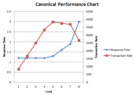
The chart shows, for each of 8 tested load levels, the response time and the transaction rate of the application.  In this case each load level is a number of concurrent requests in increments of one.  In other cases other increments may be appropriate (such as increments of 10) and other measures of load may be appropriate (message size, etc.).  Load should be driven high enough that throughput levels off.  Response time will ideally remain flat as load increases, eventually turning a knee or corner and heading upwards as capacity is reached.  In this case, the application scales nearly perfectly up to 5 concurrent requests, then begins to degrade, with peak throughput around 4,500 queries per second.

The scalability chart provides a large amount of information that can be used for capacity planning, production configuration, etc.  It shows what response times are under typical loads.  It shows the throughput capacity of a single server running the application, and it shows the behavior as capacity is exceeded.

As part of a scalability test, metrics showing server resource usage at each load level should be captured, such as CPU usage, network usage, disk usage, and memory usage.  Logs and errors should be captured.  Similar information should be captured on any downstream systems involved in the test if any, such as databases or services.

Part of the test analysis should involve bottleneck analysis, which is analyzing and determining what is limiting the capacity of the application, what is limiting it to 4,500 queries per second.  This could be server resource usage (hitting CPU, network or disk limits), it could be an increase in response time of a downstream database or server as load increases, it could be contention within the application such as thread blocking or error paths hit at high loads, etc.

An appropriate environment for a scalability test would involve two servers, one for the application and one to act as the client driving the load:

Server resource usage on the load generator should be monitored as well to verify that it is not the bottleneck.

This type of vertical scalability test does not guarantee that the application will scale out horizontally for two reasons: (1) there may be downstream systems such as databases that become bottlenecks at higher loads, and (2) load balancing or clustering systems may not scale as expected.  More extended testing beyond a minimal plan would have to cover these factors as well.

For the vertical scalability test, it is important to drive the application up to peak capacity, regardless of what expected load may be.  Usage may be different than expected, spikes in load may occur, business might grow, etc.  Some performance or stability problems only manifest themselves at higher loads, and it is important to identify these even if production load is expected to be much lower.

2. Stability

The second part of the minimal load test plan is the stability test.  To verify stability, a high load should be run against the application for an extended period of time, at a minimum 24 hours and ideally for days or weeks.  A high load can be determined from the results of the scalability test, just below peak capacity, just below the point at which response time takes a turn for the worse.  In the example above, a load of 5 concurrent requests could be used, assuming those are the final results following resolution of performance bottlenecks.

During the run, server resource usage should be captured and monitored, and error logs monitored, as with the scalability test.  Trends should be monitored closely.  Does response time degrade over time?  That indicates a resource leak.  Does CPU usage increase over time?  That indicates a design or implementation error.  Does memory leak?  Do errors begin to occur at some point or occur in some pattern?  Does the application eventually crash?

Beyond the Minimal Plan

Beyond the minimal plan, other tests are required to ensure the application is completely performant and stable.  These will be covered later (http://sub-second.blogspot.com/2011/11/extending-load-test-plan.html) and include:

1. Performance regression
2. Horizontal scalability
3. Fault tolerance